This guide covers what mixed-model production scheduling actually is, why it matters, how to execute it step by step, and where most operations get it wrong.
Key Takeaways
- Mixed-model scheduling sequences different product variants on a shared line to balance workload and minimize waste
- It implements the lean principle of heijunka — producing to the actual demand mix rather than in large batch quantities
- The core process covers takt time calculation, workload-smoothing sequencing, and building a finite schedule around real constraints
- Sequence-dependent setup times and real-time disruptions are the hardest factors to manage simultaneously
- Spreadsheets and basic ERP tools can't model these constraints; complex environments require finite scheduling software
What Is Mixed-Model Production Scheduling?
Mixed-model production scheduling is the discipline of planning the exact sequence and timing of multiple product variants — each with different work content, materials, and options — on a single shared assembly line, in a way that meets demand while protecting line efficiency.
The goal is to sequence those variants so work content stays balanced across stations over time, idle time is minimized, and output rate matches what customers are actually ordering — not just to share floor space between products.
How It Differs from Related Concepts
These terms get conflated. Here's how they actually differ:
- Mixed-model production — the system design decision to run multiple variants on one line
- Mixed-model scheduling — the daily operational execution of what to build, in what sequence, and when
- Line balancing — the upstream design task of assigning work content to stations to minimize imbalance
Scheduling is the execution layer. A well-balanced line still fails if the sequence is wrong. A good schedule can only do so much if the line is poorly balanced in the first place. Getting one right without the other leaves performance on the table — which is why treating them as a single problem is where most mixed-model implementations run into trouble.
Why Mixed-Model Production Scheduling Matters
Modern customers want product variety and short lead times at the same time. That combination kills batch production economics. Running large batches of a single model generates finished goods inventory that doesn't match the actual demand mix — and the floor space, carrying costs, and lead times that come with it.
What Happens Without Proper Scheduling
On unscheduled or batch-scheduled mixed-model lines, the symptoms are predictable:
- WIP accumulates between stations as faster models create local congestion
- Some workstations sit idle while others are consistently overloaded
- Finished goods pile up in variants customers haven't ordered yet
- Changeovers cluster unpredictably, compressing actual productive time
A 2019 study of a mixed-model combi-boiler assembly line measured this directly: station-level changeover losses totaled 149 seconds per product transition, with 46 lost units per day before sequencing improvements were applied. After sequencing changes, transition time dropped from 240 to 120 seconds for one product family, and lost devices fell to 34 per day.
The Lean Foundation: Heijunka
Mixed-model scheduling is the operational mechanism that implements heijunka, the Toyota Production System principle of leveling both the volume and variety of production over time. As the Lean Enterprise Institute defines it, heijunka means distributing production evenly so output matches demand without large batch fluctuations.
For automotive, aerospace, consumer electronics, and furniture manufacturers running hundreds of variants on shared lines, this isn't a lean preference. It's a practical necessity. BMW's production network assembles different drivetrain types and model variants on single lines across all its locations. Porsche Leipzig builds Panamera plug-in hybrid variants alongside Macan and Cayenne models on shared flexible lines. The scheduling discipline behind that is what keeps throughput stable.
How Mixed-Model Production Scheduling Works
The process follows a logical sequence: understand demand, calculate the production rate, sequence jobs to smooth workload, then build a schedule that accounts for every real constraint on the floor.
Step 1: Define Demand Mix and Takt Time
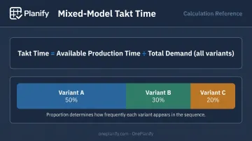
Takt time is calculated as total available production time divided by total customer demand across all variants. In a mixed-model environment, the formula extends across the full product mix:
Takt Time = Available Production Time ÷ Total Demand (all variants)
Each variant gets a demand proportion — say, 50% / 30% / 20% of the total mix — which determines how frequently it must appear in the sequence. Individual variants will have cycle times above or below the overall takt. That's expected. The scheduler's job is to sequence them so the average throughput at each station aligns with takt over time.
Step 2: Sequence Products to Balance Workload
Sequencing is where scheduling decisions have the most direct impact on floor performance. The objective, as described in mixed-model assembly research, has two goals: smooth workload at each workstation and maintain a consistent usage rate for parts and materials.
In practice, this means:
- Alternating high-work-content variants with low-work-content variants to prevent station overload
- Avoiding consecutive runs of the same model family when setup times apply
- Grouping variants that share similar tooling or fixture requirements to reduce total changeover time
- Using sequence logic that prevents blockage (upstream station finishes faster than downstream can absorb) and starvation (downstream station waits on upstream)
A simple example: scheduling a high-option variant (more assembly steps) followed by a low-option variant (fewer steps) gives the overloaded station from the first job time to recover before the next high-content unit arrives.
Step 3: Build and Execute the Finite Schedule
The sequenced job list becomes a detailed, time-based schedule — assigning jobs to specific machines, operators, and time slots while accounting for:
- Shift start and end times
- Planned maintenance windows
- Inter-operation dependencies (job B can't start until job A completes)
- Real setup times between consecutive jobs
A purpose-built finite scheduling tool is essential here. Finite scheduling respects actual capacity constraints from the start — it won't assign two jobs to the same resource at the same time, and it accounts for setup transitions rather than ignoring them. OnePlanify is designed for exactly this environment: mixed-model schedules with variable setup times, shift constraints, and cross-job dependencies that quickly exceed what spreadsheet formulas can track.
Once the schedule is live, execution requires real-time feedback. Machine breakdowns, material shortages, and operator absences are daily realities. The schedule needs to be adjustable when conditions change — which is what finite scheduling software enables and static spreadsheets cannot.
Key Factors That Affect Mixed-Model Scheduling in Practice
Process Time Variability
The wider the spread of work content across variants, the harder it is to keep stations balanced. Scheduling several high-work-content models consecutively creates work congestion and incomplete tasks — a pattern documented consistently in mixed-model sequencing research. Higher variability in processing times makes both blockage and starvation more likely, directly reducing throughput.
Sequence-Dependent Setup Times
When switching from one product variant to another requires tooling changes, fixture adjustments, or program updates, the order in which jobs run determines how much productive time gets consumed by changeovers. Setup matrices need to be treated as a first-class scheduling input — not something reconciled after the sequence is built.
The 2024 research on bipartite sequence-dependent setup times in mixed-model synchronous assembly lines confirms that optimizing launch intervals around setup dependencies directly reduces downtime and energy use.
Line Balancing Quality
No scheduling logic compensates for a poorly balanced line. If one station consistently carries more work than the others regardless of sequence — it's a bottleneck by design. Scheduling can reduce how often that station is hit with back-to-back high-content jobs, but it can't eliminate the structural imbalance. Assembly Magazine notes that a well-balanced line typically maintains a balance delay below 5%; lines exceeding that threshold will show throughput constraints that sequencing alone won't solve.
Operator Flexibility and Cross-Training
Some variants require different skills at specific stations. A schedule built on the assumption that any operator can perform any task will break down the moment that assumption is tested. Workforce flexibility is a direct input to scheduling feasibility — the more cross-trained the workforce, the more sequencing options the planner has.
Real-Time Disruption Handling
Machine breakdowns, quality holds, and absenteeism hit every busy shop floor — regularly, not occasionally. A mixed-model schedule that can't be quickly revised when disruptions occur will cascade into WIP buildup and missed deliveries. That gap separates finite scheduling — which respects real capacity and re-runs against current conditions — from a simple sequence list that goes stale within hours of the shift starting.
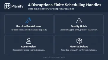
Key disruption scenarios finite scheduling must handle:
- Machine breakdowns: Re-sequence affected jobs around available capacity without rebuilding the entire plan
- Quality holds: Isolate flagged units and reschedule downstream work to prevent line starvation
- Absenteeism: Reassign tasks based on actual operator availability and cross-training records
- Material delays: Shift launch order to prioritize jobs with confirmed material on hand
Common Misconceptions and Limitations
Misconception: Optimal scheduling means a repeating cycle pattern
Many teams default to a fixed A-B-C-A-B-C sequence and call it mixed-model scheduling. The optimal sequence actually changes every day — it shifts based on demand mix, current setup states, operator availability, and machine condition. A rigid repeating cycle ignores real constraints and often performs worse than a dynamically generated finite schedule.
The tool used to build that schedule matters just as much as the logic behind it.
Spreadsheets and basic ERP sequencing modules schedule from due dates and then reconcile capacity afterward (or skip reconciliation entirely). They don't model setup times between consecutive jobs, shift transition constraints, or inter-operation dependencies. The result is a schedule that looks feasible on a screen but creates chaos on the floor. Planners spend their shift reacting to problems rather than executing a plan.
That said, mixed-model scheduling isn't the right fit for every operation. Consider a different approach when:
- Products share virtually no process steps or equipment — separate dedicated lines may have lower coordination overhead
- Demand for individual variants changes unpredictably day to day — scheduling effort may not yield stable enough plans to execute
- The product mix requires fundamentally different routings — a job shop configuration with different scheduling logic may fit better
The clearest warning sign cuts across all of these scenarios: if the shop floor team already knows "the schedule" is wrong before the shift starts, the scheduling method isn't matched to the actual complexity of the environment.
Frequently Asked Questions
What is the difference between mixed-model production and batch production?
Batch production manufactures large quantities of a single product before switching to the next, building up finished goods inventory along the way. Mixed-model production runs different variants continuously on the same line in smaller quantities, aligning output more closely with actual customer demand and reducing the inventory that builds up waiting to be ordered.
What is heijunka and how does it relate to mixed-model scheduling?
Heijunka is the lean principle of leveling production volume and variety over time so output matches demand without large batch swings. Mixed-model scheduling is how heijunka gets implemented operationally: sequencing different variants across the day or week to match the demand mix without building inventory in any single model.
How do you calculate takt time in a mixed-model environment?
The overall line takt time is total available production time divided by total demand across all variants. Individual variants will have different actual cycle times — some above takt, some below. The scheduler's job is to sequence them so the average throughput rate at each station aligns with the overall takt over time.
What is the biggest challenge in mixed-model production scheduling?
Managing sequence-dependent setup times and real-time disruptions simultaneously. Most scheduling approaches handle one reasonably well but not both. The result is schedules that are accurate at shift start but outdated by mid-morning, leaving planners reacting to the floor instead of directing it.
Is mixed-model scheduling only practical for high-volume manufacturers like automotive plants?
No. Automotive is the most visible application, but mixed-model scheduling applies equally in mid-volume job shops, electronics assembly, furniture manufacturing, and aerospace. Any environment where two or more product variants share equipment and operators benefits from structured sequencing, regardless of production volume.
How does setup time affect mixed-model production scheduling?
Sequence-dependent setup times are one of the most significant constraints in any mixed-model schedule. Ordering jobs so similar variants flow through logical changeover sequences — rather than alternating between dissimilar models — can recover substantial productive capacity. Ignoring the setup matrix when sequencing is one of the fastest ways to lose output time.