
Introduction
Picture an anti-lock braking system that calculates the correct wheel pressure — but delivers that result 50 milliseconds too late. The calculation was right. The timing wasn't. The result is the same as no response at all.
This is the core principle of real-time systems: a correct result delivered too late is a failed result. Timing correctness isn't secondary to functional correctness — it is functional correctness.
The 1997 Mars Pathfinder mission illustrated this directly. A priority inversion bug caused a high-priority task to miss its deadline, triggering repeated full system resets and delaying science data collection. The hardware was fine, the logic was sound — but the scheduling was broken.
That failure mode isn't unique to spacecraft. It shows up anywhere timing constraints govern outcomes. This guide covers:
- What real-time scheduling is and how it's measured
- Hard, soft, and firm real-time systems
- Major scheduling algorithms (RMS, EDF)
- Static vs. dynamic approaches
- How these principles translate directly to manufacturing shop floors
Key Takeaways
- In real-time systems, timing is part of correctness — a late result is a wrong result
- Hard real-time systems treat any deadline miss as failure; soft systems tolerate occasional lateness
- Rate Monotonic Scheduling uses static priorities; EDF uses dynamic priorities and achieves higher CPU utilization
- Manufacturing scheduling mirrors OS scheduling: jobs have deadlines, machines have finite capacity, and disruptions demand dynamic re-prioritization
- Static production plans become obsolete the moment conditions change; dynamic rescheduling is the practical reality
What Is Real-Time Scheduling?
Real-time scheduling is the discipline of determining the order and timing of task execution so every task completes within its specified deadline — not eventually, but at the right moment.
This distinguishes it from general-purpose scheduling, which optimizes for throughput or fairness. Real-time scheduling optimizes for timing guarantees.
The Three Metrics That Matter
| Metric | Definition |
|---|---|
| Timeliness | How closely actual completion matches the deadline |
| Predictability | How consistent timing behavior is across executions |
| Feasibility | Whether the full task set can be scheduled within all constraints |
A system can be timely on average but unpredictable in worst-case scenarios — which is unacceptable in flight control or industrial machinery.
Interrupt Latency and Dispatch Latency
Real-time systems are event-driven: they wait for hardware signals, timer expirations, or sensor data, then respond within bounded time. Two delays determine how fast that response actually happens:
- Interrupt latency: time from hardware interrupt assertion to the first instruction of the interrupt handler
- Dispatch latency: time from the last instruction of the interrupt service routine to when the readied thread begins executing
Both must be bounded and accounted for in any schedulability analysis. On a real-time Linux kernel, cyclictest benchmarks show maximum latencies in the range of 65–141 microseconds — with actual worst-case values in production environments running higher depending on hardware and load conditions.
Hard vs. Soft Real-Time Systems
Not all deadlines carry the same consequences when missed. Understanding which category your system falls into determines which algorithms and verification approaches are appropriate.
Hard Real-Time
Any deadline miss constitutes a system failure — regardless of how small the violation.
Examples include flight control systems, anti-lock braking, medical device controllers, and industrial machinery. A guidance system that responds 10 milliseconds late is as dangerous as one that never responds. There's no partial credit.
Soft Real-Time
Missed deadlines degrade performance but don't cause system failure. The system recovers and continues operating.
Video streaming is the classic example. A dropped frame produces a visual glitch. Audio playback with occasional buffer underruns produces a click. Neither is catastrophic, and the system self-corrects.
Firm Real-Time
This category sits between the two. A result delivered after its deadline has zero value — but the miss itself doesn't cause catastrophic failure.
Consider a trading system that computes an optimal order price: if the calculation finishes after the trading window closes, the result is worthless, but the system doesn't crash. Firm systems don't require the mathematical proof of deadline guarantees that hard systems demand, but they also can't rely on soft-system tolerances — making them a distinct design category with their own tradeoffs.
| System Type | Missed Deadline Effect | Failure Risk | Example |
|---|---|---|---|
| Hard | System failure | Catastrophic | Anti-lock braking, flight control |
| Firm | Result becomes worthless | Non-catastrophic | Trading order execution |
| Soft | Performance degrades | None | Video streaming, audio playback |

Key Real-Time Scheduling Algorithms
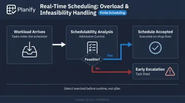
Before executing a task set, a real-time scheduler performs schedulability analysis — a pre-runtime determination of whether all deadlines can be guaranteed. If the answer is no, the scheduler rejects the task rather than accepting it and failing at runtime — a mechanism called admission control.
Two algorithms dominate real-time scheduling theory and practice.
Rate Monotonic Scheduling (RMS)
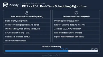
RMS assigns static priorities inversely proportional to task period: shorter period, higher priority. The schedule is fixed at design time and never changes during execution.
Liu & Layland's 1973 paper proved that RMS is optimal among fixed-priority schedulers. If any fixed-priority assignment can schedule a task set, RMS can.
Schedulability bound:
A task set is guaranteed schedulable if:
Σ(Cᵢ/Tᵢ) ≤ n(2^(1/n) − 1)
As n grows large, this bound converges to approximately 69%. That's the ceiling — RMS cannot guarantee full CPU utilization even when it's theoretically available.
Key implications:
- Priorities are simple to assign and understand
- Behavior is predictable under overload
- CPU utilization ceiling limits efficiency at high loads
Earliest Deadline First (EDF)
EDF assigns priorities dynamically: at every scheduling decision point, the runnable task with the nearest absolute deadline gets the CPU. Priorities recalculate continuously as tasks arrive and deadlines change.
Liu & Layland proved EDF achieves 100% CPU utilization while guaranteeing all deadlines on a uniprocessor — something RMS fundamentally cannot do.
That theoretical advantage comes with real tradeoffs:
- Dynamic priority recalculation introduces runtime overhead
- Under overload conditions, which tasks miss deadlines becomes less predictable than with RMS
- Implementation complexity is higher
When utilization stays comfortably below 69%, both algorithms deliver. Push above that threshold and EDF's dynamic flexibility becomes the deciding factor.
Other Algorithm Classes
Three additional approaches appear in embedded systems:
- Static table-driven scheduling — a fixed schedule computed entirely at design time, used in simple pipeline systems where the workload never changes
- Dynamic best-effort scheduling — no feasibility guarantee; tasks are simply aborted if deadlines are missed, common in systems where occasional misses are acceptable
- Server-based scheduling — sporadic or aperiodic tasks are handled by a dedicated server with its own budget, preserving the schedulability guarantees of the underlying RMS or EDF framework
Static vs. Dynamic Scheduling Approaches
The algorithm choice connects to a broader architectural decision: when are scheduling decisions made?
Static scheduling determines all task priorities and execution orders before the system runs, based on task characteristics defined at design time. It works well when the workload is fully defined and stable — simple embedded control loops being the classic case. Predictability is high; flexibility is low.
Dynamic scheduling determines priorities at runtime in response to changing conditions. It handles variable workloads and unexpected events better, but requires more computational overhead and introduces less predictability in worst-case timing.
The Manufacturing Parallel
This distinction maps directly to shop floor operations:
- A static production plan is built the night before based on known orders, machine assignments, and shift schedules. It assumes nothing changes.
- A dynamic schedule continuously re-prioritizes work orders based on machine availability, material readiness, operator presence, and shifting due dates.
Research on dynamic manufacturing scheduling confirms the practical reality: in real manufacturing environments, unexpected events are inevitable, and static schedules based on estimates can become obsolete immediately after release to the floor.
That gap between plan and reality is precisely why most modern production environments rely on some form of dynamic re-scheduling — and why the underlying algorithm matters as much as the scheduling software itself.
Real-Time Scheduling in Manufacturing and Shop Floor Operations
Manufacturing scheduling shares the fundamental real-time property: timing correctness matters independently of functional correctness.
A job started too early ties up a machine needed for a higher-priority order. A job started too late causes downstream starvation or a missed customer commitment.
The "deadline" in manufacturing is the customer due date or the next downstream operation's start window. Missing either has the same consequence as a late interrupt response in a control system.
Finite Capacity Scheduling as Schedulability Analysis
Finite capacity scheduling is the manufacturing equivalent of schedulability analysis. Rather than assuming unlimited machine capacity, the scheduler enforces actual constraints:
- One machine can only run one job at a time
- Shift changes reduce available hours in defined windows
- Setup times between jobs consume real capacity
- Inter-job dependencies create sequencing constraints
Cambridge IfM defines finite capacity scheduling as scheduling that considers capacity from the outset — directly contrasting it with MRP-style infinite scheduling, which schedules from due dates and then tries to reconcile with capacity after the fact. That reconciliation step is where plans fall apart.
Disruptions as Interrupt Events
Machine breakdowns, material shortages, operator absences, and quality holds are the manufacturing equivalent of interrupt latency — unpredictable events that force immediate re-prioritization of the entire task queue.
The Siemens/Senseye True Cost of Downtime 2022 report found that unplanned downtime costs industrial manufacturers an average of $129 million per facility annually — with automotive operations losing over $2 million per hour of unplanned stoppage. Static scheduling offers no defense against this.

When a critical machine goes down at 8 a.m., the plan from the night before doesn't reschedule itself. A shop floor manager must manually re-sequence work orders, recalculate dependencies, and identify which customer commitments are now at risk — all while production sits idle.
Dynamic Rescheduling in Practice
A 2023 case study in the thermoplastics industry found that dynamic shop-floor scheduling using real-time information reduced tardiness by 26.1% and total weighted cost by 6.99% compared to static approaches. The mechanism is the same as EDF: when new deadline information arrives, re-prioritize immediately rather than executing a stale plan.
Translating that principle into daily operations requires tools designed for shop floor complexity, not theoretical models. OnePlanify handles setups, shift changes, inter-job dependencies, and live disruptions within a finite scheduling framework — without requiring a dedicated scheduling specialist. The result is the same dynamic response that makes EDF effective in control systems: real constraints captured, stale plans replaced the moment conditions change.
Key capabilities that support this include:
- Finite capacity enforcement across all work centers
- Automatic re-sequencing when disruptions occur
- Dependency tracking to prevent downstream starvation
- Shift and setup constraints built into every schedule
Challenges of Real-Time Scheduling and How to Address Them
Overhead and Context Switching
Every scheduling decision costs time. In computing systems, frequent preemption can itself cause deadline misses — research on interrupt accounting shows that release overhead for global EDF implementations can exceed 50 microseconds worst-case, with costs scaling as task set size grows.
In manufacturing, the equivalent cost is planner time. Constantly re-sequencing manually is unsustainable and introduces human error at exactly the moment when accuracy matters most.
How to address it: Choose scheduling granularity appropriate to the system's volatility. Don't reschedule every five minutes if conditions only meaningfully change every few hours.
Overload and Infeasibility
When more work arrives than can be completed by all deadlines, something has to give. The scheduler must decide what to shed:
- In computing: abort lower-priority tasks
- In manufacturing: escalate infeasible commitments to operations leadership before the deadline, not after
The key word is before. Admission control exists precisely to detect overload conditions early. Discovering a schedule is infeasible at runtime, or on the morning a shipment is due, is a failure of the planning process, not just bad luck.
Verification and Worst-Case Analysis
For hard real-time systems, schedulability must be mathematically proven under worst-case execution times (WCET), not average cases. Wilhelm et al. define WCET as an upper bound on execution times required for schedulability analysis — average performance is not a safe planning assumption when a single miss constitutes system failure.
For manufacturing, this translates to stress-testing schedules against plausible disruption scenarios before releasing them to the floor. What happens if the primary machine for a critical job goes down at 7 a.m.? The answer should be known in advance.
Complexity vs. Usability
Advanced scheduling algorithms often require deep expertise to configure and maintain. The practical challenge for manufacturing operations is finding an approach that captures real constraints (finite capacity, setups, dependencies) without requiring a specialist to run it every day.
That gap between theoretically optimal and actually used is where most scheduling tools fail shop floors. OnePlanify is built to close it: finite scheduling that handles real production complexity without requiring an engineer to operate it daily.
Frequently Asked Questions
What is RT in process scheduling?
"RT" stands for Real-Time, referring to scheduling policies where tasks must execute within strict timing constraints. In Linux, RT scheduling classes — SCHED_FIFO and SCHED_RR — give real-time tasks preemptive priority over standard processes. SCHED_FIFO runs without time slicing; SCHED_RR adds a round-robin quantum within the same priority level.
What is the difference between hard and soft real-time scheduling?
Hard real-time systems treat any deadline miss as a system failure — flight control and ABS braking are typical examples. Soft real-time systems tolerate occasional misses with degraded but recoverable performance, such as video streaming.
What is the difference between Rate Monotonic Scheduling and Earliest Deadline First?
RMS assigns static priorities based on task period (shorter period = higher priority) and is optimal among fixed-priority algorithms, but caps schedulable CPU utilization at approximately 69%. EDF assigns dynamic priorities based on current deadlines and can theoretically achieve 100% CPU utilization, though with higher runtime overhead and less predictable behavior under overload.
What is finite scheduling in manufacturing?
Finite scheduling accounts for real capacity limits — machines, labor, and time — when building a production schedule. Unlike infinite scheduling (used in MRP), it ensures no two jobs are assigned to the same resource simultaneously and that setup times and shift constraints are respected.
How does real-time scheduling apply to manufacturing operations?
Manufacturing jobs have deadlines (due dates, downstream operation windows), machines have finite capacity analogous to CPU time, and disruptions like breakdowns or material shortages require dynamic rescheduling. This mirrors the re-prioritization EDF performs when new deadline information arrives.
What happens when a real-time system is overloaded and cannot meet all deadlines?
The scheduler must shed work — aborting lower-priority tasks in computing, or escalating infeasible commitments before they're missed in manufacturing. Admission control and schedulability analysis exist to detect overload early, enabling deliberate trade-offs before options run out.